One-Off Analysis Scripts: Cycling Torque Example

This tutorial shows you how to build a one-off analysis script in minutes with SweatStack. We will build a script that fetches your cycling data (road and trainer), and calculates and plots simple power-cadence and torque-cadence relationships.

What You'll Build

A Python script that:

• Is completely standalone
• Fetches your cycling data (road vs trainer)
• Calculates torque from power and cadence
• Visualizes the relationships

Setup

Make sure you have uv installed for running Python scripts with inline dependencies.

Create a new file analysis.py with inline dependencies and the required imports:

analysis.py

# /// script
# requires-python = ">=3.10"
# dependencies = [
#     "sweatstack",
#     "pandas",
#     "numpy",
#     "matplotlib",
# ]
# ///

import os
from datetime import date

import sweatstack as ss
import pandas as pd
import numpy as np
import matplotlib.pyplot as plt

The # /// script format lets you run the script directly with uv run analysis.py - no requirements.txt file needed!

Authentication

Add authentication to your script:

analysis.py

# /// script
# requires-python = ">=3.10"
# dependencies = [
#     "sweatstack",
#     "pandas",
#     "numpy",
#     "matplotlib",
# ]
# ///

import os
from datetime import date

import sweatstack as ss
import pandas as pd
import numpy as np
import matplotlib.pyplot as plt

# Authenticate (opens browser once, then cached)
ss.authenticate()

This opens your browser once to authenticate. Your credentials are saved for future use.

Just try it out with uv run analysis.py to see how it works.

Fetching Longitudinal Data

SweatStack's get_longitudinal_data fetches time-series data across multiple activities:

analysis.py

# ... previous code omitted ...

ss.authenticate()

# Fetch all road cycling power and cadence data
road_cycling_data = ss.get_longitudinal_data(
    sport=ss.Sport.cycling_road,
    start=date(2024, 1, 1),
    metrics=["power", "cadence"],
)

# Fetch trainer data for comparison
trainer_cycling_data = ss.get_longitudinal_data(
    sport=ss.Sport.cycling_trainer,
    start=date(2024, 1, 1),
    metrics=["power", "cadence"],
)

This returns DataFrames with all your power and cadence data indexed by timestamp.

Enable Caching for Development

When exploring your data, you'll often run the same script several times. To save time, you can cache your data so you don't have to download it from the API every run. Just turn on caching and set a fixed end date—this way, you always get the same data and your results are reproducible.

analysis.py

# ... previous code omitted ...

ss.authenticate()

# Enable caching to avoid re-fetching data
os.environ["SWEATSTACK_LOCAL_CACHE"] = "true"

# Fetch all road cycling power and cadence data
road_cycling_data = ss.get_longitudinal_data(
    sport=ss.Sport.cycling_road,
    start=date(2024, 1, 1),
    end=date(2025, 1, 1),  # Fixed end date for caching
    metrics=["power", "cadence"],
)

# Fetch trainer data for comparison
trainer_cycling_data = ss.get_longitudinal_data(
    sport=ss.Sport.cycling_trainer,
    start=date(2024, 1, 1),
    end=date(2025, 1, 1),  # Fixed end date for caching
    metrics=["power", "cadence"],
)

Cache Tip

Always set an explicit end date when caching - using date.today() would create new cache entries daily!

Calculating Torque

Add a function to calculate torque from power and cadence:

analysis.py

# ... previous code omitted ...

# Fetch data
road_cycling_data = ss.get_longitudinal_data(
    sport=ss.Sport.cycling_road,
    start=date(2024, 1, 1),
    end=date(2025, 1, 1),
    metrics=["power", "cadence"],
)

trainer_cycling_data = ss.get_longitudinal_data(
    sport=ss.Sport.cycling_trainer,
    start=date(2024, 1, 1),
    end=date(2025, 1, 1),
    metrics=["power", "cadence"],
)

# Calculate torque (Nm) = Power (W) / Angular velocity (rad/s)
def calculate_torque(power, cadence):
    angular_velocity = cadence * (2 * np.pi / 60)  # Convert RPM to rad/s

    torque = pd.Series(index=power.index)
    mask = angular_velocity > 0  # Avoid division by zero
    torque[mask] = power[mask] / angular_velocity[mask]

    return torque

# Add torque column to both datasets
road_cycling_data["torque"] = calculate_torque(
    road_cycling_data["power"], 
    road_cycling_data["cadence"]
)
trainer_cycling_data["torque"] = calculate_torque(
    trainer_cycling_data["power"], 
    trainer_cycling_data["cadence"]
)

Creating Visualizations

Now add the plotting code to visualize the relationships:

analysis.py

# ... previous code omitted ...

# Add torque column to both datasets
road_cycling_data["torque"] = calculate_torque(
    road_cycling_data["power"], 
    road_cycling_data["cadence"]
)
trainer_cycling_data["torque"] = calculate_torque(
    trainer_cycling_data["power"], 
    trainer_cycling_data["cadence"]
)

# Create comparison plots
fig, [cadence_power_plot, cadence_torque_plot] = plt.subplots(2, 1, figsize=(10, 10))

# Plot 1: Cadence vs Power
cadence_power_plot.scatter(
    road_cycling_data["cadence"],
    road_cycling_data["power"],
    color="red", marker=".", alpha=0.5,
    label=ss.Sport.cycling_road.display_name(),
)
cadence_power_plot.scatter(
    trainer_cycling_data["cadence"],
    trainer_cycling_data["power"],
    color="blue", marker=".", alpha=0.5,
    label=ss.Sport.cycling_trainer.display_name(),
)
cadence_power_plot.set_xlabel("cadence [rpm]")
cadence_power_plot.set_ylabel("power [W]")
cadence_power_plot.legend()

# Plot 2: Cadence vs Torque  
cadence_torque_plot.scatter(
    road_cycling_data["cadence"],
    road_cycling_data["torque"],
    color="red", marker=".", alpha=0.5,
    label=ss.Sport.cycling_road.display_name(),
)
cadence_torque_plot.scatter(
    trainer_cycling_data["cadence"],
    trainer_cycling_data["torque"],
    color="blue", marker=".", alpha=0.5,
    label=ss.Sport.cycling_trainer.display_name(),
)
cadence_torque_plot.set_xlabel("cadence [rpm]")
cadence_torque_plot.set_ylabel("torque [Nm]")
cadence_torque_plot.legend()

plt.show()

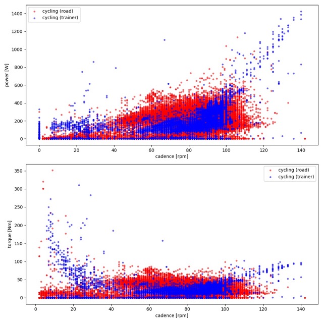
The result looks like this:

Run Your Analysis

uv run analysis.py

That's it! In less than 100 lines, you've built a complete power analysis comparing road and trainer cycling.

View complete code

# /// script
# requires-python = ">=3.10"
# dependencies = [
#     "sweatstack",
#     "pandas",
#     "numpy",
#     "matplotlib",
# ]
# ///

import os
from datetime import date

import sweatstack as ss
import pandas as pd
import numpy as np
import matplotlib.pyplot as plt

os.environ["SWEATSTACK_LOCAL_CACHE"] = "true"

ss.authenticate()

def calculate_torque(power, cadence):
    """
    Calculate torque from power and cadence
    Torque (Nm) = Power (W) / (Cadence (rpm) × 2π/60)
    """
    angular_velocity = cadence * (2 * np.pi / 60)

    torque = pd.Series(index=power.index)
    mask = angular_velocity > 0
    torque[mask] = power[mask] / angular_velocity[mask]

    return torque

road_cycling_data = ss.get_longitudinal_data(
    sport=ss.Sport.cycling_road,
    start=date(2024, 1, 1),
    end=date(2025, 1, 1),
    metrics=["power", "cadence"],
)

trainer_cycling_data = ss.get_longitudinal_data(
    sport=ss.Sport.cycling_trainer,
    start=date(2024, 1, 1),
    end=date(2025, 1, 1),
    metrics=["power", "cadence"],
)

road_cycling_data["torque"] = calculate_torque(
    road_cycling_data["power"], 
    road_cycling_data["cadence"]
)
trainer_cycling_data["torque"] = calculate_torque(
    trainer_cycling_data["power"], 
    trainer_cycling_data["cadence"]
)

fig, [cadence_power_plot, cadence_torque_plot] = plt.subplots(2, 1, figsize=(10, 10))

cadence_power_plot.scatter(
    road_cycling_data["cadence"],
    road_cycling_data["power"],
    color="red", marker=".", alpha=0.5,
    label=ss.Sport.cycling_road.display_name(),
)
cadence_power_plot.scatter(
    trainer_cycling_data["cadence"],
    trainer_cycling_data["power"],
    color="blue", marker=".", alpha=0.5,
    label=ss.Sport.cycling_trainer.display_name(),
)
cadence_power_plot.set_xlabel("cadence [rpm]")
cadence_power_plot.set_ylabel("power [W]")
cadence_power_plot.legend()

cadence_torque_plot.scatter(
    road_cycling_data["cadence"],
    road_cycling_data["torque"],
    color="red", marker=".", alpha=0.5,
    label=ss.Sport.cycling_road.display_name(),
)
cadence_torque_plot.scatter(
    trainer_cycling_data["cadence"],
    trainer_cycling_data["torque"],
    color="blue", marker=".", alpha=0.5,
    label=ss.Sport.cycling_trainer.display_name(),
)
cadence_torque_plot.set_xlabel("cadence [rpm]")
cadence_torque_plot.set_ylabel("torque [Nm]")
cadence_torque_plot.legend()

plt.show()